install.packages("usethis") #if you haven't already installed
library(usethis)

usethis::create_github_token()

gitcreds::gitcreds_set()Reproducible workflows
This is a walkthrough example of how we might go about producing a reproducible piece of research.
There are several steps to this:
- We all need to create a Github account.
- We get our computer talking to Git by logging our Github credentials (either SSH or HTTPS approach)
- We create a Github Repo
- We create an R “Project”
- We start writing our code
- We “commit” and then “push” our changes when ready
- Once everything is complete, we write up in Markdown format
Setting up Github credentials
Once we’ve got our Github account, we’re ready to get our computer talking to Github. We do this in the following way:
And you can do this directly in RStudio like this:
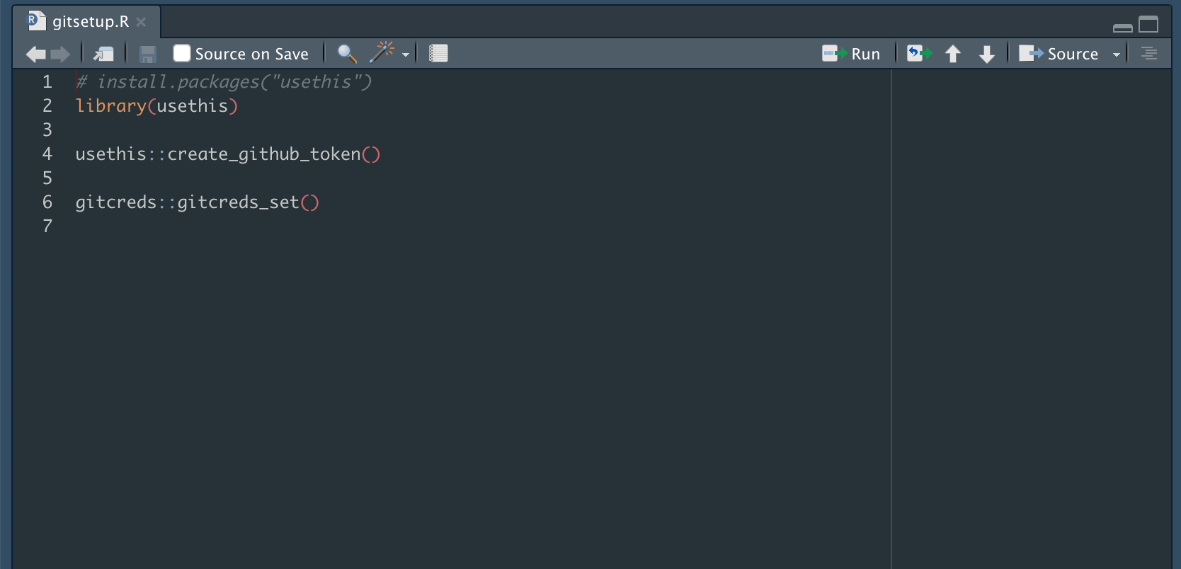
You log your credentials there and you’re all set.
Creating a Github Repo
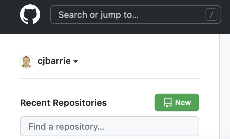
We first need to use our Github account (that we made in step one) by creating a “Repo.” This is just the place where we’re going to be logging and storing all our code and materials.
To do this, we go on to our Github account a select “New” next to the “Recent Repositories” tab. Mine looks like this:
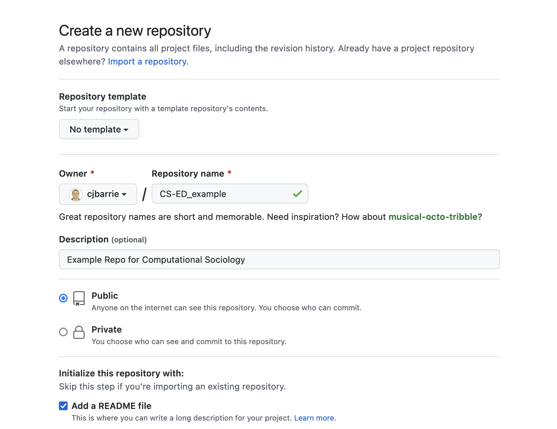
Once we’ve done that, we can name and describe our Repo as below. We also add a “README,” which will be a kind of landing page online but will serve as the main explainer file should anyone want to download and reproduce your research.
We then press Create and you’ll be redirected to your new repository:
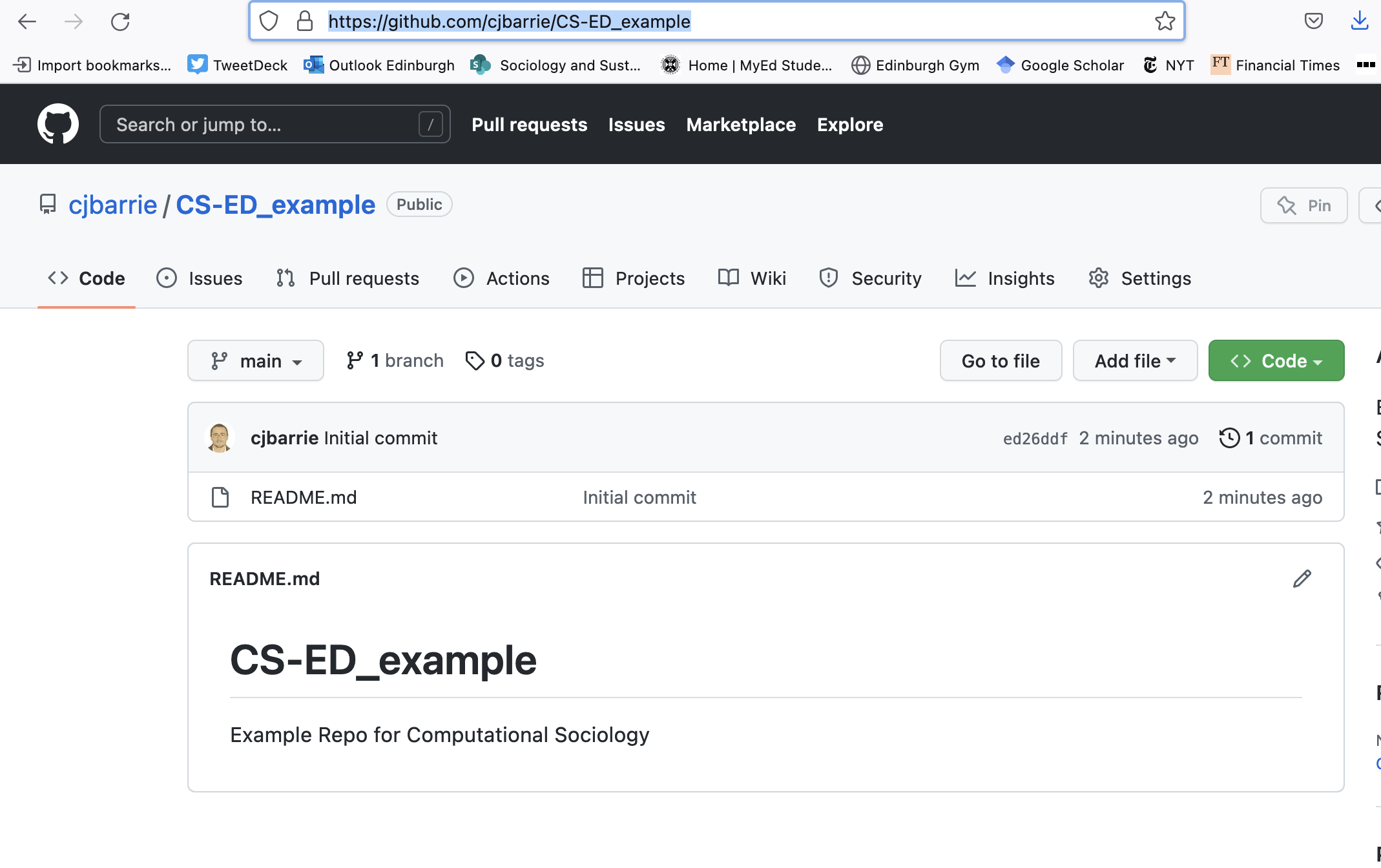
You’re ready for the next step!
Creating an R Project
Next we create an R Project by selection File –> New Project.
You’ll see a window like this pop up:

And you should select Version Control, whereupon you’ll be asked:
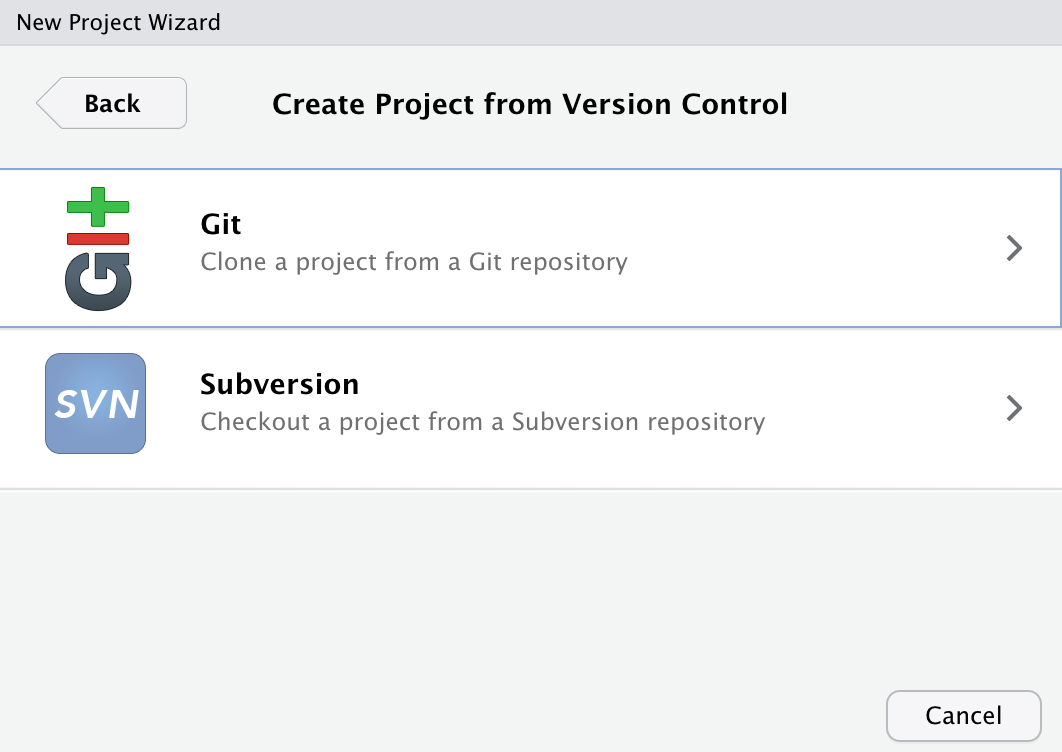
to choose either Git or Subversion. Choose Git. Then you’ll be asked to put in the name of the URL of the Github Repo you’ve created.
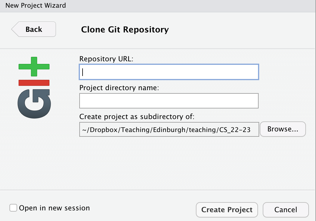
And here we will enter the URL of the Github Repo we just created: https://github.com/cjbarrie/CS-ED_example.
We start writing our code
Now that we’re in our new R Project, we can start adding some contents!
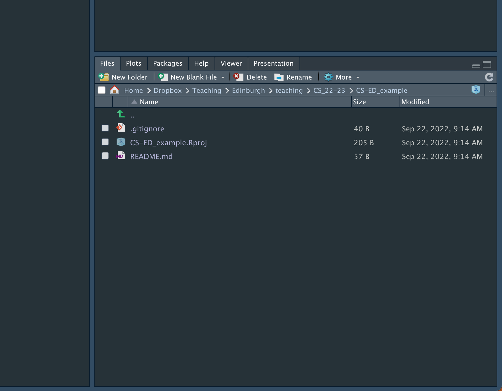
At the start, your directory will look something like this:
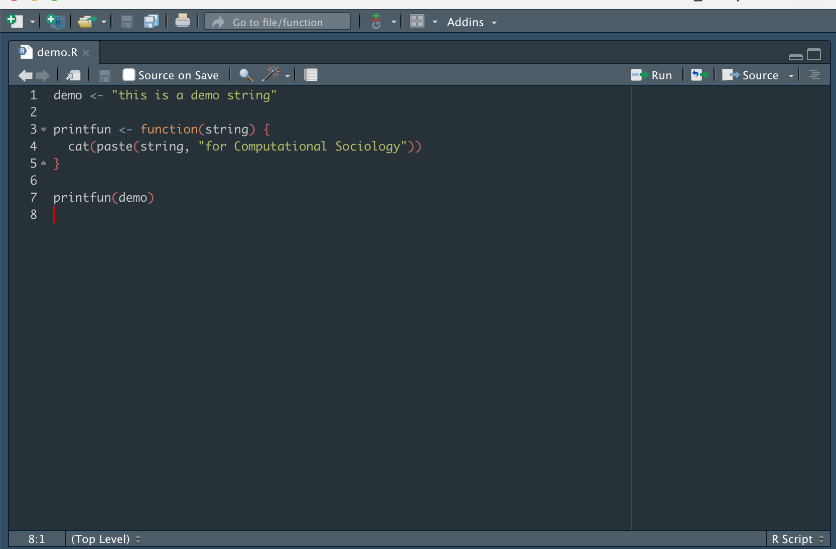
We add a new script by pressing the top left icon of some white paper with a green + sign next to it. Or we can go to File –> New File –> R Script.
Here I’m just writing a dummy example where I write a pointless function that prints a string followed by “for Computational Sociology.”
Once we’ve done this we can “Commit” and “Push.” And remember when we Commit we describe what this “Commit” (basically a version at which you’ve placed a yard stick or marker) is doing. Here I write that I am adding the first script.
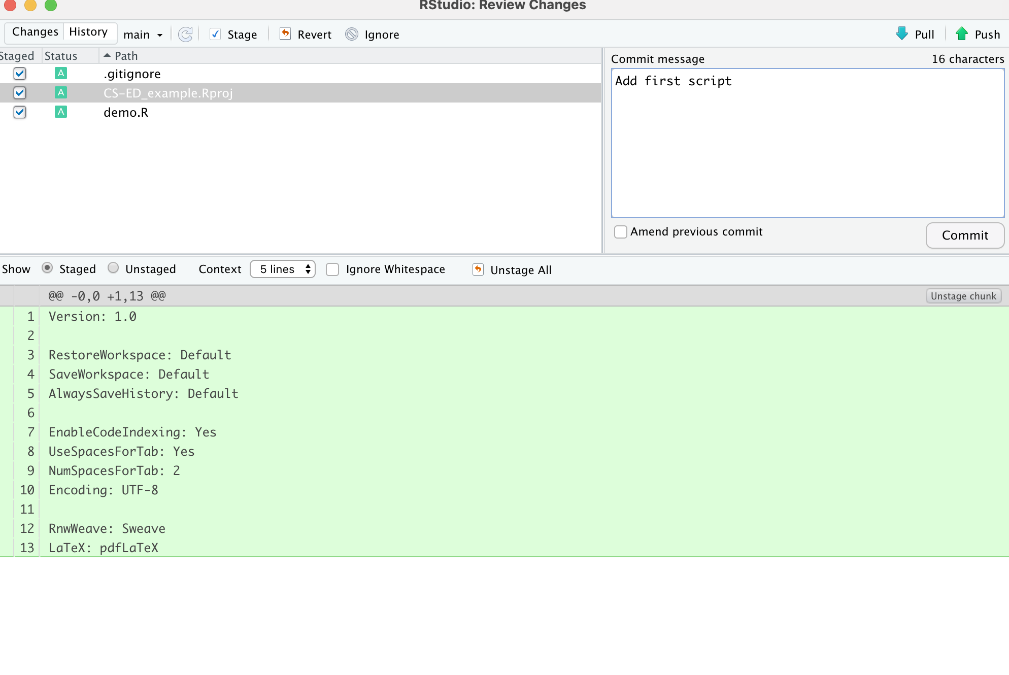
Then commit and push to our Github Repo we’ve set up within this R Project.
At which point we can go back to our “Remote” version of our work (the version that’s hosted on Github) and see if the changes are recorded there:
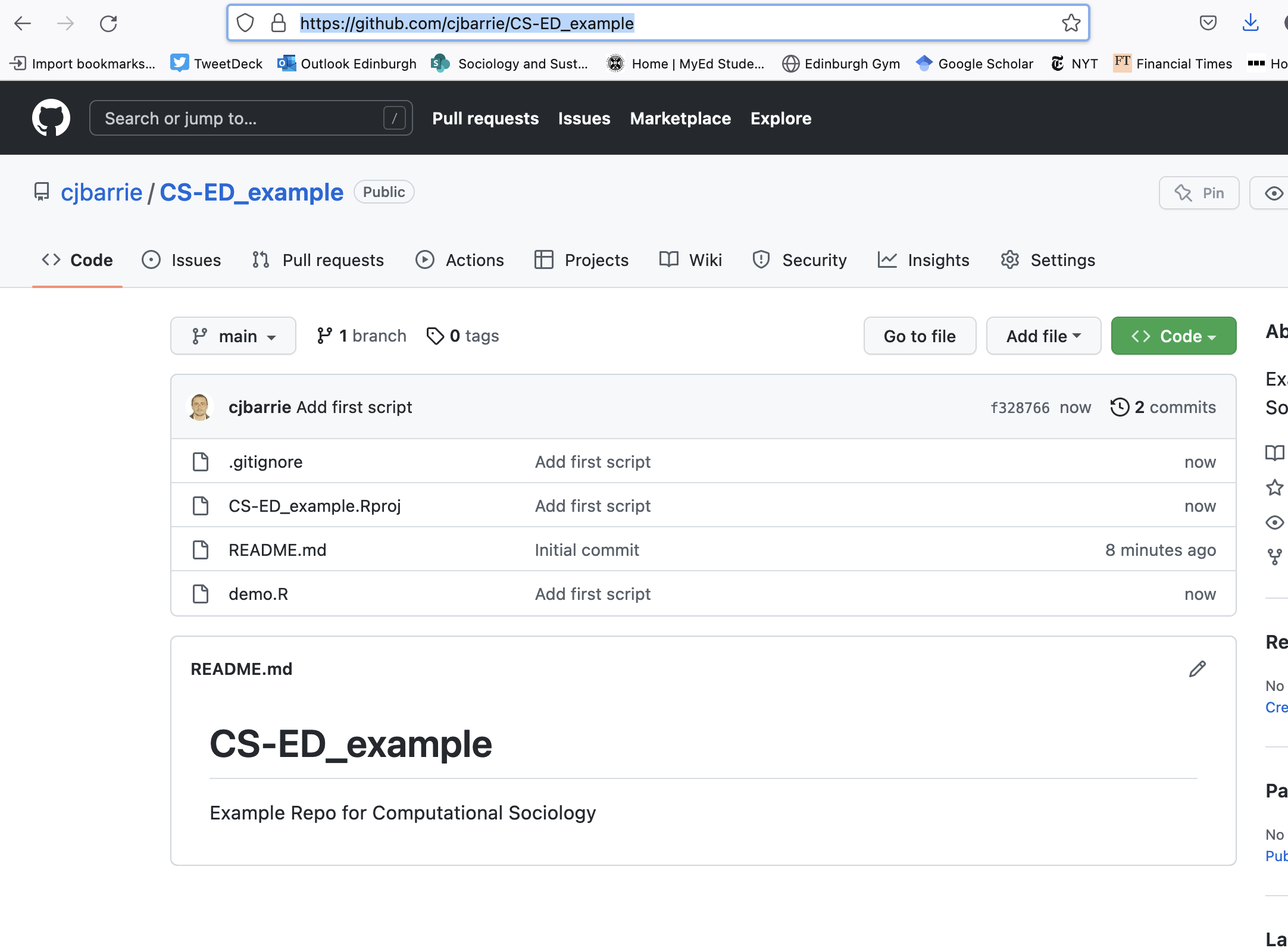
Ta da! Congratulations: you’re on your to producing reproducible research :).
Writing up in Markdown
Let’s say we want to answer one of the questions in Worksheet 1.
We’d first open our R Project that we’ve already linked to Github by following the steps above.
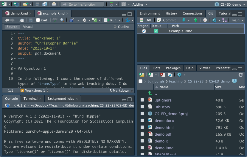
Within this project, we’d then open a new .Rmd file as follows, selecting the pdf output format and naming it “Worksheet 1”.
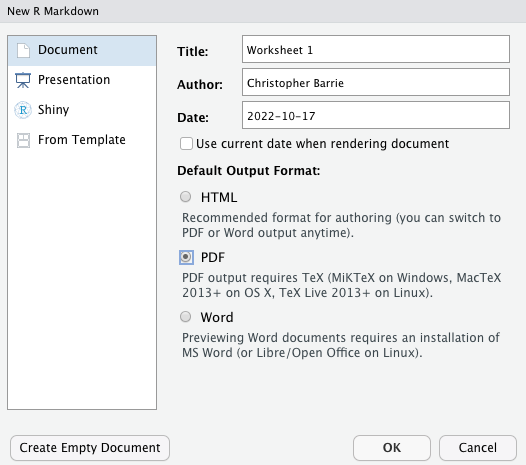
We’ll be met with a document that looks something like this:
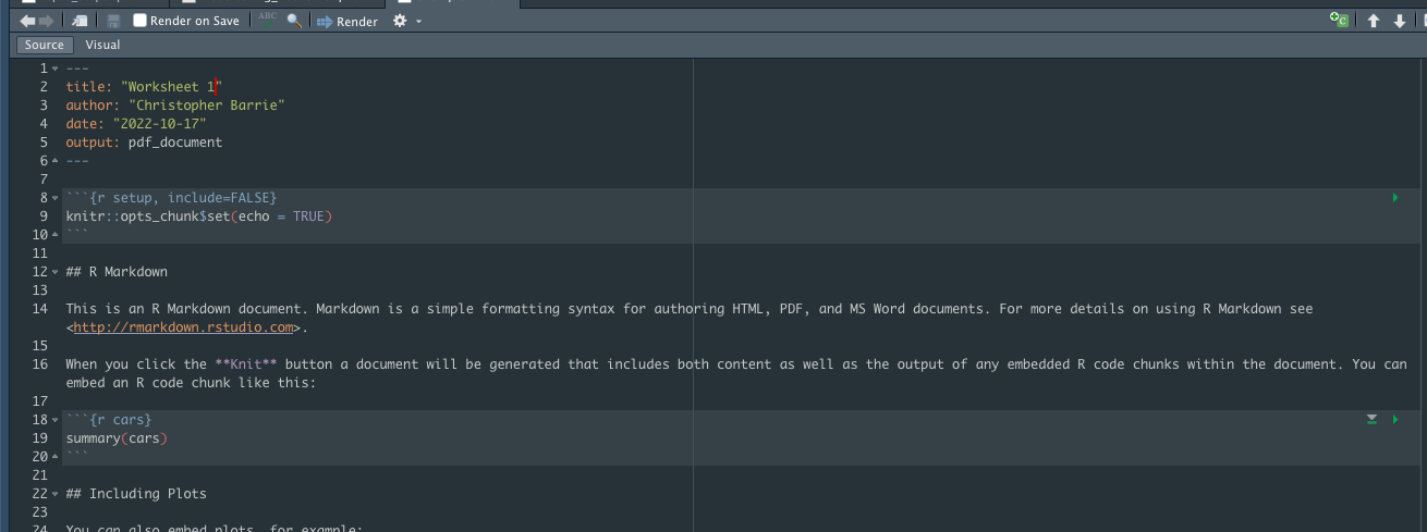
The section that reads
knitr::opts_chunk$set(echo = TRUE)is just setting some default display options, e.g., the formatting of figure sizes and other optional typesetting parameters. We normally don’t need to worry about this—and these can also be set for each specific chunk of code (rather than as global defaults). You can read more about these here.
We can therefore remove all of the template content in order to add our own markdown:

And we can now begin to add our answers by inserting our first code chunk. We can also describe what we did above it.
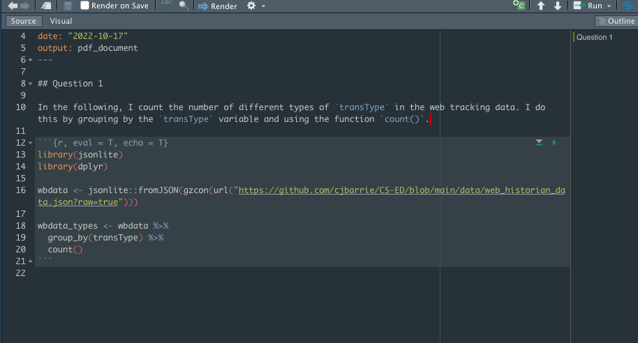
Note that here we’re using eval = T and echo = T as we want our code to appear in the markdown output and to be computed (rather than just printed). When we set eval = T, we are telling our machines to run the code specified; when we specify echo = T, we are telling out machines to print the code in the pdf (or html or word) output.
Now that we’re down, we can press “Render,” which will produce our pdf document.
We can now “Commit” and “Push” to Github to store this version of our work remotely.
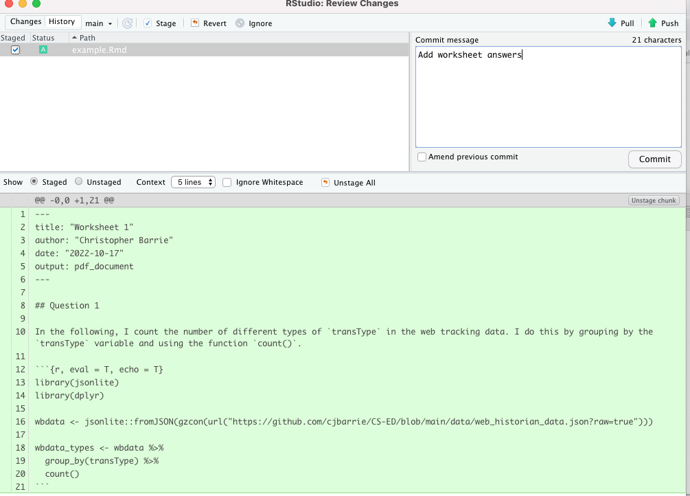
After which we should see it on our remote version as below:
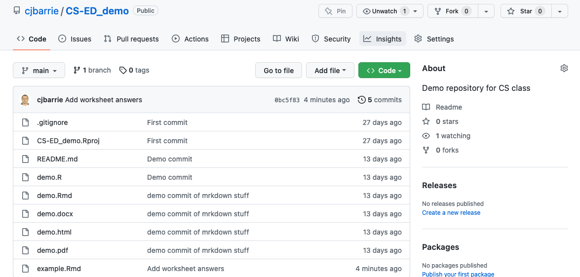
And we’re done! Now just rinse and repeat…